At defcon24 this year, I impulsively bought myself some new toys. Amongst what I got included a YARD Stick One and a Ubertooth One. I already owned a DVB-T dongle much like this one that I bought at defcon23 the previous year.
My interest in Software Defined Radio has long been one of those where I just felt so overwhelmed with the idea for a very long time that I dare not try it. This, together with the fact that its something I totally know nothing about really did make for this bit of research to be pretty daunting at first.
Nonetheless, here is my adventure into reverse engineering a plain static key remote and successfully replaying it from my computer.
the terminology
Where to start? In hindsight, I guess a sane point of departure would have been to first figure out what all of these new acronyms mean. OOK, PWM, AM, FSK etc were all things I have only seen but never actually knew what they meant. I read a whole bunch of blog posts and other RTL-SDR related stuff, thinking I could just dive right in. It was not long before I realized that its pretty important when someone talks about Pulse Width Modulation(PWM) that I actually know that this means!
So, as I progressed through the resources I found online, I made a note of looking up the acronyms and what the general idea behind them were. The most important of the acronyms you should know is listed below. You should seriously take some time to look into these in more detail and not just rely on my silly descriptions:
-
AM - Amplitude Modulation
When talking AM, we are referring to the fact that the signal strength (or amplitude) is varied according to the waveform that is being transmitted. This gif shows a comparison between AM and FM (Frequency Modulation) for the same signal. It should be clear that for the same signal, AM increases the amplitude of the waveform, and FM increases the frequency of the waveform -
PWM - Pulse Width Modulation
In addition to AM, in the case of these static key remotes, they make use of PWM. Basically, the duration of a pulse determines the bit that is being send. A long pulse is a zero, and a short pulse is a one. -
OOK - On-off keying
On-off keying is a form of Amplitude-shift keying where a binary value is represented based on the duration of the presence of a carrier signal (or a just a high amplitude signal).
the gear
Once I had a good idea of what all of this stuff means, it was time to get some gear to play with. I went to a local electronics store to pick up a few things. The most important being a static key remote. I also needed something that will switch on when the remote is pressed. For this, I settled on a small LED light, just to give an indication of life. All in all I must have spent close to R600 (~40USD) for everything. The list of lab toys included:
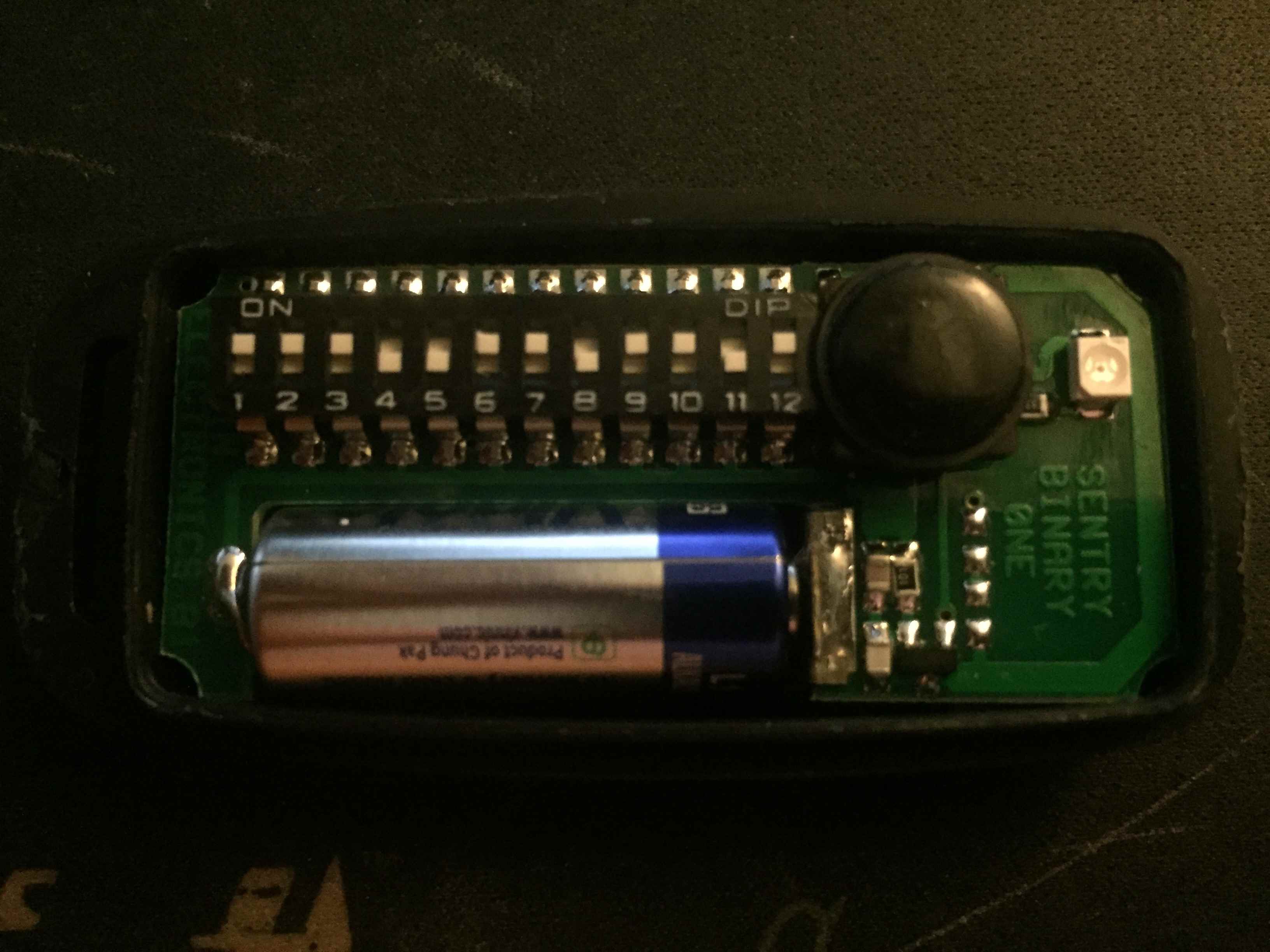
- 1 x Basic 433Mhz Binary Code Transmitter
- 1 x 12V Power Supply
- 1 x Generic, Static Key Receiver
- 1 x 10W LED Light (wow this thing is bright!)
- 1 x Enclosure
- Some wiring etc.
I setup, wired together and tested everything. The LED light was wired up to the normally open contact so that when the remote button is pressed, the light will go on for a brief period of time and then switch off.
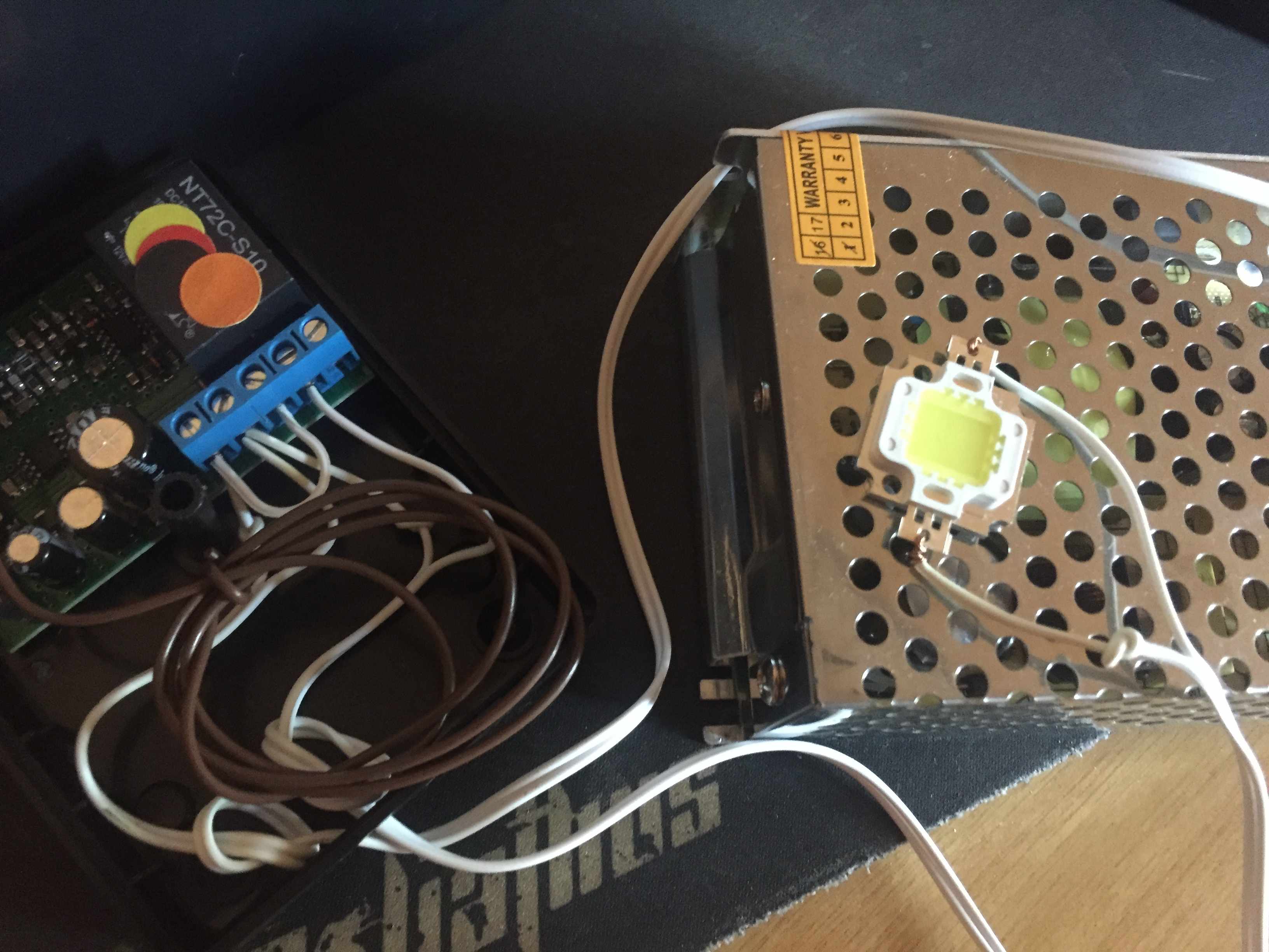
I paired my remote with a random position of the 12 dip switches on it to the receiver and tested that the light actually goes on under normal conditions. Sweet.
the signal capture
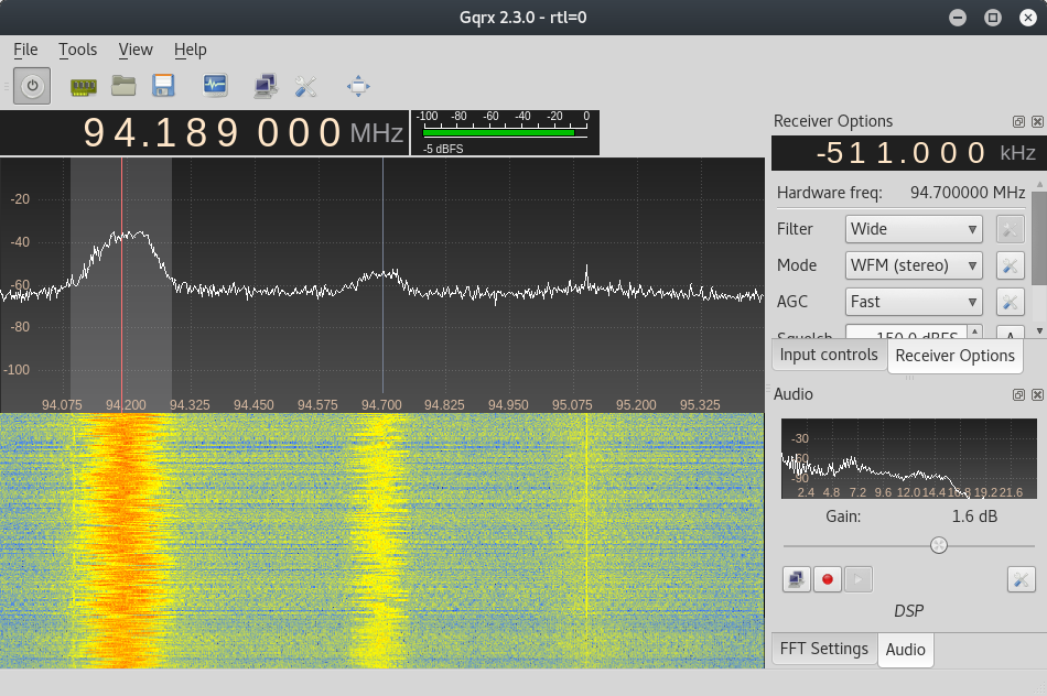
Capturing the remotes signal turned out to be a little easier than I initially expected. I found plenty of resources online that helped me get familiar with ways to do it. The most common capture method I could see was to use a tool called GXRQ. GQRX allows you to tune into the frequency and make a raw recording of the signal to file. This is probably the fastest way to get the recordings to file. The recorded file can then be opened up in gnuradio or inspectrum. You can do a number of fun things with GQRX, like listening to radio! (I had to enable Hardware AGC in GQRX for this to work) :)
Anyways. I got stuck trying to decode the key from the remote using a GQRX recording. No matter how I loaded it into inspectrum or audacity (or even raw parsing attempts at some stage), I just could not make head or tail of what I was looking at. In fact, it all just turned out to be garbage to me. Maybe because I didn’t set it to record AM? Who knows. Anyways.
the gnuradio reveal
Speaking to @elasticninja (thanks for your epic patience dude!), I got tipped off to an absolutely great video by Michael Ossmann in he’s Software Defined Radio with HackRF series here. More specifically, lesson 8 deals with on-off keying and was excellent in getting me started with gnuradio.
This lesson does a great job of showing you how to find out more details about a specific remote that you are interested in by looking up its hardware specs, test results and any other pieces of information. It then goes on to explain how to get your first flow graph up and running in gnuradio in no time.
preparing gnuradio
Before building gnuradio flow graphs, a little bit of preparation was needed. I was using a Kali Virtual Machine in VMWare for testing and had to install a few extra packages on top of the base installation. While we on the topic of dependencies, I am just going to list everything needed to replicate that which you will find in this post:
apt install gnu-radio rfcat gr-osmosdr audacity
If you want audio to work, I had to enable pulseaudio with these commands followed by a reboot:
systemctl --user enable pulseaudio && systemctl --user start pulseaudio
With that out of the way, I was ready to replicate that flow graph from the lesson.
building the flow graph
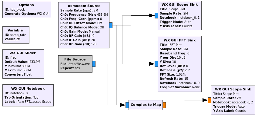
Just like the session explained, I launched gnuradio-companion and built the flow graph the same way:
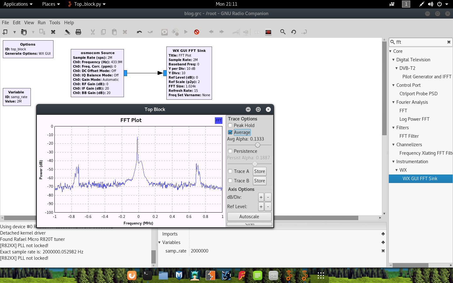
- Launch GNU radio (and start a new WX GUI Graph). I noticed it defaults to the QT GUI in the options block, so just right-click edit that and flip it over to WX GUI.
- Add a new osmocom Source block to receive data from your RTL-SDR. If you cant find the block, click on any item on the list on the right and hit ctrl-f to filter.
- Add a new WX GUI FFT Sink and connect the osmocon Source and new FFT sink by clicking on the output and input of each.
- Set a higher sample rate of 2000000 in the
samp_ratevariable by editing the Variable block. - Edit the osmocon Source block and set the RF Gain to 0 and the frequency to the one you are hoping to listen in on. In my case this is 4339e5, or 4339200000.
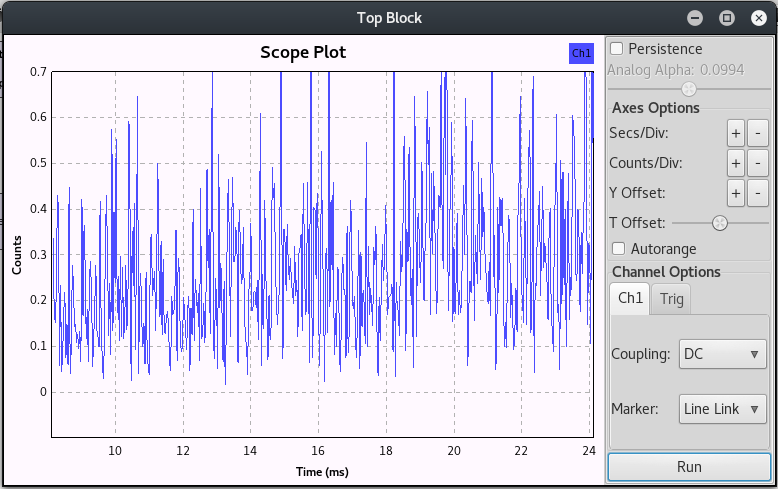
Once this is done, save the flow graph and run it (with your RTL-SDR plugged in) to visualize the signal when you press your remote!
Fast forward a bit through the lesson, and we finally get to part where we can visualize the key on the remote as a demodulated waveform with the addition of the second scope sink (around 30mins in). To get a nice and clear picture of the on-off keying, we want to measure the magnitude over time of a sample. This can be done by adding a type converter to the flow graph. The Complex to Mag type converter will do the job just fine. To add this:
- Find the type converter block called Complex to Mag and drag it onto the flow graph.
- Connect the output from the osmocon Source to the Complex to Mag input.
- Connect the output of the Complex to Mag converter to the Scope sink input.
- Change the input expected by the scope sink from complex to float.
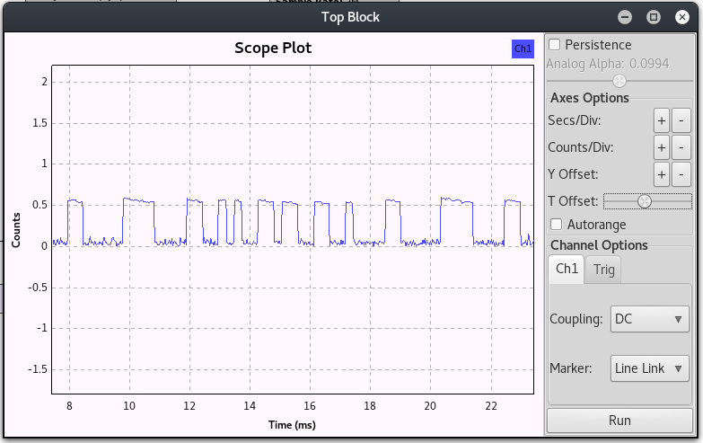
With this done, run the graph again. You will need to fiddle a little with the seconds per division and counts per division values to get the visualization just right. Unticking the Autorange box will also greatly help you narrow down the signal. As a last tip, if you experience the graph jumping around too much (from left to right), you can toggle a ‘center’ by focussing the Trig tab and setting the lines that appear with the level toggles.
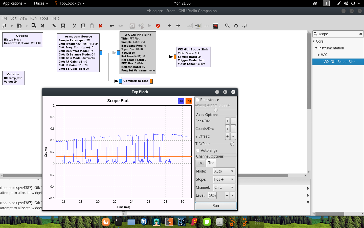
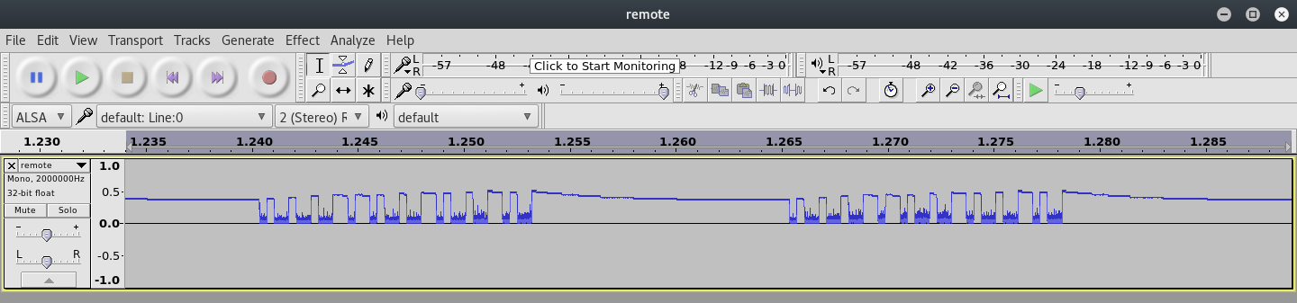
As you can see in this screenshot, the keying seems to represent the values:
[short, short, short, long, long, short, short, long, short, short, long, short]
Or:
[1, 1, 1, 0, 0, 1, 1, 0, 1, 1, 0, 1]
This indeed matches the switch positions on my remote. Yay!
storing the recordings
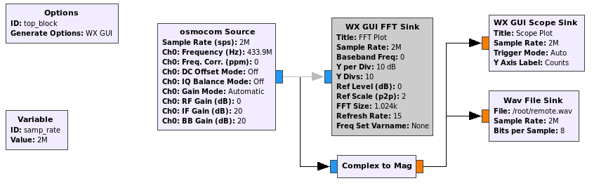
Looking at those waveforms is cool and all, but it isn’t always practical to keep your finger on a button. Instead, we can record the output to a file for later use. You may choose to record the raw, unprocessed signal from the radio (in cases where you may need to still do some processing on the file maybe?) or save the demodulated waveform. To do this, simply add a new Wave File Sink block after the Complex to Mag block and specify a destination filename.
Now, just launch the graph and press down on the remote for a while. When done, stop the graph and check if your file has been written in the location you specified:
~ # ls -lah remote.wav
-rw-r--r-- 1 root root 7.2M Oct  3 22:07 remote.wav
Great. If you need to re-use this file at a later stage in gnuradio, simply add a File Source / Wave File Source block as needed and reconnect the other blocks where appropriate.
viewing in audacity
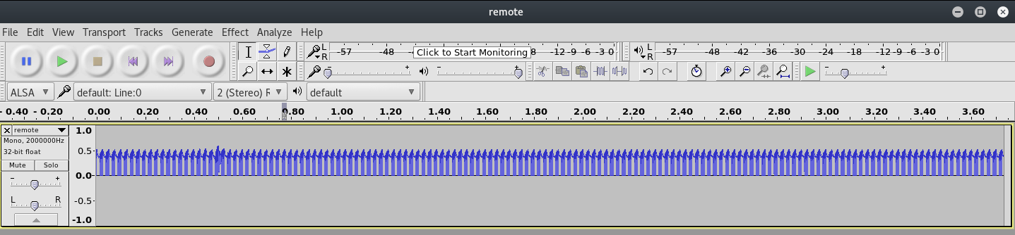
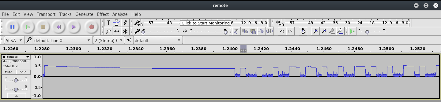
If you saved the demodulated wave file, then you can open this file in Audacity. Simply launch audacity (we already installed it) and open the recorded wave file. Viewing the recording at first may look something like this:
However, when you zoom in a little, you may start seeing the on-off keying becoming obvious:
Admittedly, getting this far was relatively easy thanks to the ton of research out there already!
introducing rfcat
I guess the main reason why I decided on the YARD Stick One was because of the fact that it comes pre-flashed with the RFcat firmware. It was only after the fact that I realized its actually a pretty good RF device in general. There are some other radios (maybe cheaper?) that you can flash to work with RFCat such as the CC1111emk dongle or the dongle that comes with the Chronos watch development kit. The RFCat wiki also has a list of compatible dongles.
As for RFcat itself, I guess the most important thing to realize is that you effectively have a python interface to the underlying radio when using it. Admittedly, there isn’t a lot of documentation for RFCat and you may very quickly come to realize that you will have to make use of the help() strings and the source code of rflib to learn the necessary. This coupled with existing projects and work online doesn’t make it too hard to get going.
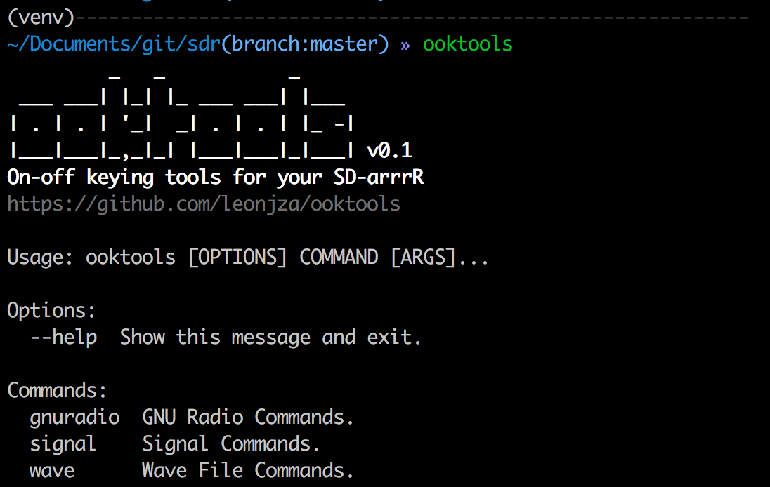
To give you an idea, below is a sample snippet of starting rfcat in ‘research’ (-r) mode and sending a string as a ‘ping’ packet. Using RFcat this way, the object d is used to call methods for the radio:
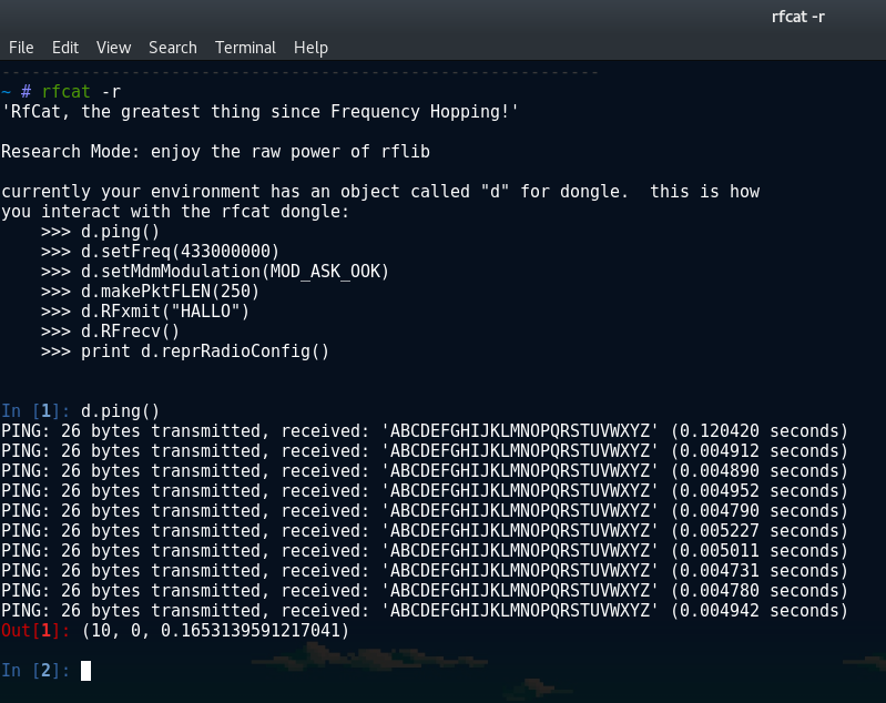
As you can see in the screenshot, there is a banner message giving you some useful hints on how you can interact with the dongle. Methods such as setFreq(), setMdmModulation() etc is all things we will be needing soon™ when we want to start replaying the signal of this remote (and switch on that very bright LED!).
sending the signal with RFcat
As you may have noticed by now, sending signals with RFCat is as simple as d.RFxmit(data='DEADBEEF'). To get the receiver to understand my replay, I didn’t think it would be as easy just playing the raw binary string of 111001101101 back. I tested anyways by writing a small script to start sending signals and then captured them using my SDR and gnuradio. The values for the frequency and baud rate is something that you should be able to get from the data sheets of the remote you are attempting to replay. (I will show you how to calculate the baud rate later though). The original script I used was:
#!/usr/bin/python

import rflib

d = rflib.RfCat()

# Set Modulation. We using On-Off Keying here
d.setMdmModulation(rflib.MOD_ASK_OOK)

d.makePktFLEN(12)    # Set the RFData packet length
d.setMdmDRate(3800)  # Set the Baud Rate
d.setMdmSyncMode(0)  # Disable preamble
d.setFreq(433920000) # Set the frequency

d.RFxmit('111001101101')
d.setModeIDLE()
I ran this script together with a gnuradio flow graph that was set up to dump the signal to a file. I then used this signal as a source to a Scope Sink that was prefixed with a Complex to Mag block. As expected, with this initial attempt I could not find anything in my graphs that even remotely looked like on-off keying!
No easy win here was ok as it forced me to dive a little into the RFCat source code in an attempt to figure out how exactly the data should be sent. I also searched online for examples of how to send data correctly and came across a number of examples to help me.
Turns out, I need to get my data into bytes to send with RFxmit(). No big deal, lets do just that!
#!/usr/bin/python

import rflib

data = '111001101101'

# Convert the data to hex
rf_data = hex(int(data, 2))

d = rflib.RfCat()

# Set Modulation. We using On-Off Keying here
d.setMdmModulation(rflib.MOD_ASK_OOK)

d.makePktFLEN(len(rf_data)) # Set the RFData packet length
d.setMdmDRate(3800)         # Set the Baud Rate
d.setMdmSyncMode(0)         # Disable preamble
d.setFreq(433920000)        # Set the frequency

# Send the data string a few times
d.RFxmit(rf_data, repeat=500)

d.setModeIDLE()
I now added the hex conversation of the original binary string and added the repeat=500 value to RFxmit() to help me find the signal with gnuradio. This was finally what I needed to be able to send data that appeared to look like on-off keying!
This was not exactly the same as the signal that I originally captured using the actual remote, but, it was progress, and I believed it to be good progress.
getting the on-off keying right
I played around quite a bit at this stage with my attempts to represent the same waveform as the ones captured from the remote I am trying to replicate. I made a major breakthrough when I came across this blog post where the author explains a method in which to accurately convert the signal into a true on-off keying waveform. The general idea being that you should take note of the smallest distance of amplitude and use that as a single binary digit. You then count the bits relative to this distance and convert to them to a 1 for a high amplitude and a 0 for a low amplitude. Effectively we are simply calculating the Pulse-width Modulation key for our binary code manually now.
So to replicate this in my example, I went back to the original wave file I recorded and extracted a single full pulse:
One important difference that I noticed with my remote compared to many similar posts I saw online was that I had this long starting high amplitude before the actual on-off keying signal started. It looked like about half of a pulse was this high amplitude, and the other half signal. I assumed these will all just be handled by adding a bunch of 1’s in front of my final key as it may have served as some form of preamble or something. ¯\_(ツ)_/¯
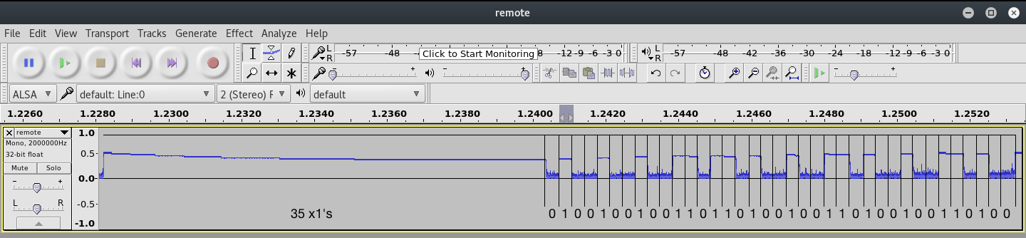
If you look closely at the above image, you would notice that the second half of the pulse is divided up into equal length sections that are of similar size as that of the smallest pulse. This size can be seen as the clock signal.
The distance of a high pulse followed by a low pulse (relative to the clock signal) signifies the bits that is being transferred. This is actually also known as Pulse-width Modulation. Applying this logic (as shown in the screenshot where the bits are filled in) to the waveform, we can deduce that the Pulse-width Modulation key (without the prefix of the 35 1’s and the 0) is:
# PWM Key version of 111001101101
100100100110110100100110100100110100
If we take an even closer look at the above PWM key, one might even notice that in relation to the waveform, the bit strings 1’s and 0’s are represented as 100 for a 1 and 110 for a 0 to form the full PWM key. We can visualize this logic in the below snippet where the PWM key is separated by a | and the original bitstring is filled in below it:
# PWM to Bitstring comparison
100 | 100 | 100 | 110 | 110 | 100 | 100 | 110 | 100 | 100 | 110 | 100
 1     1     1     0     0     1     1     0     1     1     0     1
This matches our initial bit string of 111001101101, and helps us conclude that for a full PWM key (with the leading bunch of 1’s) the resultant key would be:
# Full PWM Key
111111111111111111111111111111111110100100100110110100100110100100110100
baud rate hate
Before I get to the rest of the newly updated script, lets talk about baud rate quickly. This is something that caused me a lot of pain. I managed to get the original waveform from my remote and my generated waveform using scripts to look similar, but there was a serious issue with getting the length of the pulses to match. If you look closely at the below screenshot you will notice there is actually a problem with the key too (missing a bit), but heh, the clock signal is whats important here:
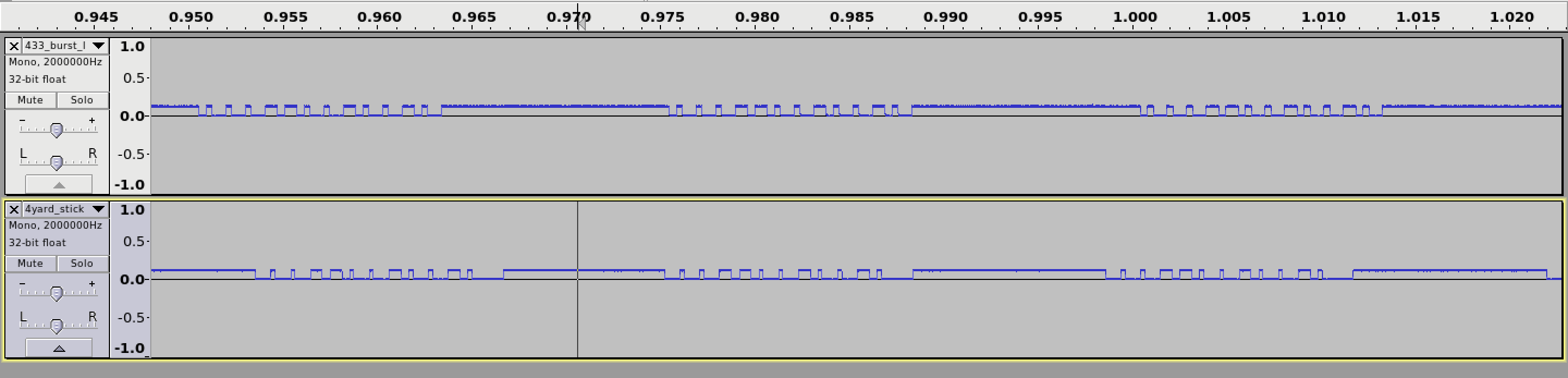
This problem existed until I finally managed to figure out what the math for the baud rate calculation was. I noticed that this value is not an exact science though. You can be off by quite a lot, and yet the signal will still have a high change of succeeding. YMMV.
Unfortunately I can not remember the post / code that lead me to this, but the basic idea for calculating baud rate is as follows:
- The source wave file would have been recorded at a certain Sample Rate. We recorded at a sample rate of 2M from gnuradio.
- We want to figure out how many samples makes up the distance of the shortest high aptitude in the pulse (much like we needed for the PWM key calculation)
- The number of samples in the shortest high amplitude bit, divided by the sample rate over 1 should give you the baud rate.
In other words:
baud = (1.0 / (length of shortest high peak / sample rate))
Practically, you can determine the values needed for the formula by opening a wave file you recorded using gnuradio, zooming and selecting one of the short pulses and changing the selection at the bottom dropdown to length and samples.
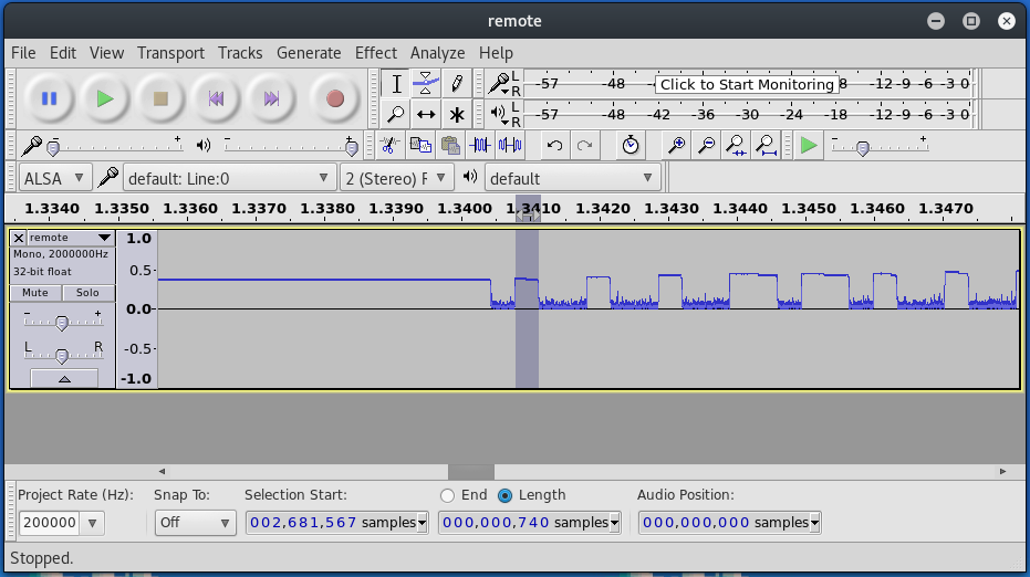
Here you can see my sample range for the shortest high peak is 740 samples, and on the far left you can see the sample rate of 2000000. That means that my baud rate will be 1.0/(740/2000000), which is ~2702 baud. Not 100% accurate, but accurate enough to work.
let there be light
One last hurdle! I had some troubles with the conversions to hex for the long bit string as a result of the PWM conversion. Thankfully, I came across the bitstring module to handle the conversion to bytes. What a fantastic library :P
The final, updated script follows:
#!/usr/bin/python

# Send a PWM String using RfCat

import rflib
import bitstring

# That prefix string. This was determined by literally
# just looking at the waveform, and calculating it relative
# to the clock signal value.
# Your remote may not need this.
prefix = '111111111111111111111111111111111110'

# The key from our static key remote.
key = '111001101101'

# Convert the data to a PWM key by looping over the
# data string and replacing a 1 with 100 and a 0
# with 110
pwm_key = ''.join(['100' if b == '1' else '110' for b in key])

# Join the prefix and the data for the full pwm key
full_pwm = '{}{}'.format(prefix, pwm_key)
print('Sending full PWM key: {}'.format(full_pwm))

# Convert the data to hex
rf_data = bitstring.BitArray(bin=full_pwm).tobytes()

# Start up RfCat
d = rflib.RfCat()

# Set Modulation. We using On-Off Keying here
d.setMdmModulation(rflib.MOD_ASK_OOK)

# Configure the radio
d.makePktFLEN(len(rf_data)) # Set the RFData packet length
d.setMdmDRate(2702)         # Set the Baud Rate
d.setMdmSyncMode(0)         # Disable preamble
d.setFreq(433920000)        # Set the frequency

# Send the data string a few times
d.RFxmit(rf_data, repeat=25)
d.setModeIDLE()
I ran this newly updated script and BAM, my labs LED light illuminates! \o/

resources
Below is basically a link dump of stuff that was super helpful in getting as far as I did with this. These posts may help clear things up that made no sense in this post!
General On-off keying stuff:
- http://andrewmohawk.com/2012/09/06/hacking-fixed-key-remotes/
- https://zeta-two.com/radio/2015/06/23/ook-ask-sdr.html
- http://www.rtl-sdr.com/using-a-yardstick-one-hackrf-and-inspectrum-to-decode-and-duplicate-an-ook-signal/
- https://blog.compass-security.com/2016/09/software-defied-radio-sdr-and-decoding-on-off-keying-ook/
- http://leetupload.com/blagosphere/index.php/2014/02/24/non-return-to-zero-askook-signal-replay/
- http://adamsblog.aperturelabs.com/2013/03/you-can-ring-my-bell-adventures-in-sub.html
- http://dani.foroselectronica.es/rfcat-ti-chronos-and-replaying-rf-signals-337/
Sample code:
- https://github.com/AndrewMohawk/RfCatHelpers
- https://github.com/ade-ma/LibOut/blob/master/scripts/rfcat-libout.py
- https://github.com/alextspy/rolljam/blob/master/rf_car_jam.py
further work
With that done, I set off to write a toolkit that allows you to work with rfcat and On-off keying data sources such as wave files, or just simple recordings from rfcat itself. After finishing the polishing, I’ll release it along with a post detailing its internals and usage! In the meantime, keep an eye on this repository https://github.com/leonjza/ooktools
Happy hacking!